Matrix Multiplication

Table of Contents

• Problem Formulation
• Parallel Decomposition
• Benchmarking

We study parallel 2D matrix multiplication on a CPU, showing how Taskflow's parallel-for algorithm turns a sequential triple-nested loop into a scalable parallel program with minimal code change.

Problem Formulation

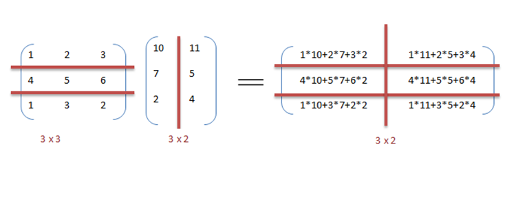
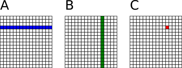
We multiply matrix A (M×K) by matrix B (K×N) to produce output matrix C (M×N). The number of columns in A must equal the number of rows in B. Each element C[m][n] is the dot product of row m of A and column n of B:

The sequential triple-nested loop is:

for(int m = 0; m < M; m++) {
  for(int n = 0; n < N; n++) {
    C[m][n] = 0;
    for(int k = 0; k < K; k++) {
      C[m][n] += A[m][k] * B[k][n];
    }
  }
}

Parallel Decomposition

The rows of C are completely independent of one another — computing row m does not affect any other row. We exploit this independence by assigning one task per row. This coarse-grained decomposition gives each task enough work to amortise the overhead of task creation and scheduling:

void matrix_multiplication(int** A, int** B, int** C, int M, int K, int N) {
  tf::Taskflow taskflow;
  tf::Executor executor;
 
  // one task per row of C
  for(int m = 0; m < M; m++) {
    taskflow.emplace([m, &]() {
      for(int n = 0; n < N; n++) {
        for(int k = 0; k < K; k++) {
          C[m][n] += A[m][k] * B[k][n];
        }
      }
    });
  }
 
  executor.run(taskflow).wait();
}

The same parallelism can be expressed more concisely using tf::Taskflow::for_each_index, which handles partitioning and scheduling automatically:

taskflow.for_each_index(0, M, 1, [&](int m) {
  for(int n = 0; n < N; n++) {
    for(int k = 0; k < K; k++) {
      C[m][n] += A[m][k] * B[k][n];
    }
  }
});

See Parallel Iterations for partitioning strategies and chunk-size tuning that can further improve performance.

Benchmarking

The table below compares sequential and parallel CPU runtimes on a 12-core Intel i7-8700 at 3.2 GHz:

Matrix size	CPU sequential	CPU parallel
10×10	0.142 ms	0.414 ms
100×100	1.641 ms	0.733 ms
1000×1000	1532 ms	504 ms
2000×2000	25688 ms	4387 ms
3000×3000	104838 ms	16170 ms
4000×4000	250133 ms	39646 ms

For small matrices the task-creation overhead dominates and the sequential version is faster. As the matrix size grows, task overhead becomes negligible relative to the computation, and the parallel speed-up grows toward the number of available cores — reaching 6.3× at 4000×4000.

Note

For GPU-accelerated matrix multiplication that achieves over 90× speed-up at large sizes, see Matrix Multiplication with CUDA GPU.